Subsections

• 12.2.1 The Model
• 12.2.2 Firing time distribution
• 12.2.3 Stationary Synaptic Weights
• 12.2.4 The Role of the Firing Threshold

12.2 Learning to be Precise

We have seen in Section 12.1 that learning rules with an asymmetric learning window can selectively strengthen those synapses that reliably transmit spikes at the earliest possible time before the postsynaptic neuron gets activated by a volley of spikes from other presynaptic neurons. This mechanism may be relevant to speed up the information processing in networks that contain several hierarchically organized layers.

Here we are going to discuss a related phenomenon that may be equally important in networks that are based on a time-coding paradigm, i.e., in networks where information is coded in the precise firing time of individual action potentials. We show that an asymmetric learning window can selectively strengthen synapses that deliver precisely timed spikes at the expense of others that deliver spikes with a broad temporal jitter. This is obviously a way to reduce the noise level of the membrane potential and to increase the temporal precision of the postsynaptic response (Kistler and van Hemmen, 2000a).

12.2.1 The Model

We consider a neuron i that receives spike input from N presynaptic neurons via synapses with weights w_ij, 1$\le$j$\le$N. The membrane potential u_i(t) is described by the usual SRM₀ formalism with response kernels $\epsilon$ and $\eta$, and the last postsynaptic firing time $\hat{{t}}_{i}^{}$, i.e.,

$$\eta \hat{{t}}_{i}^{} \sum_{{\substack{j=1 \\ (j\ne i)}}}^{N} \int_{0}^{\infty} \epsilon$$ (12.1)

Postsynaptic spikes are triggered according to the escape-noise model (Section 5.3) with a rate $\nu$ that is a nonlinear function of the membrane potential,

$$\nu \nu_{{\text{max}}}^{} \Theta \vartheta$$ (12.2)

If the membrane potential is below the firing threshold $\vartheta$, the neuron is quiescent. If the membrane potential reaches the threshold, the neuron will respond with an action potential within a characteristic response time of $\nu_{{\text{max}}}^{{-1}}$. Note that the output rate is determined by the shape of the $\eta$ kernel rather than by $\nu$(u). In particular, the constant $\nu_{{\text{max}}}^{}$ is not the maximum firing rate but the reliability of the neuron. The larger $\nu_{{\text{max}}}^{}$ the faster the neuron will fire after the firing threshold has been reached. For $\nu_{{\text{max}}}^{}$$\to$$\infty$ we recover the sharp firing threshold of a noiseless neuron model. We refer to this neuron model as the nonlinear Poisson model.

Presynaptic spike trains are described by inhomogeneous Poisson processes with a time-dependent firing intensity $\nu_{i}^{}$(t). More specifically, we consider a volley of spikes that reaches the postsynaptic neuron approximately at time t₀. The width of the volley is determined by the time course of the firing intensities $\nu_{i}^{}$. For the sake of simplicity we use bell-shaped intensities with a width $\sigma_{i}^{}$ centered around t₀. The width $\sigma_{i}^{}$ is a measure for the temporal precision of the spikes that are conveyed via synapse i. The intensities are normalized so that, on average, each presynaptic neuron contributes a single action potential to the volley.

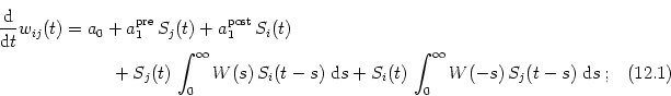
Synaptic plasticity is implemented along the lines of Section . Synaptic weights change whenever presynaptic spikes arrive or when postsynaptic action potentials are triggered,

$$\begin{multline} \frac{{\text{d}}}{{\text{d}}t} w_{ij}(t) = a_0 + a_1^{\text{pr... ...s + S_i(t) \, \int_0^\infty W(-s) \, S_j(t-s) \; {\text{d}}s \,; \end{multline}$$

cf. Eqs. (10.14)-(10.15). In order to describe Hebbian plasticity we choose an asymmetric exponential learning window W that is positive for s < 0 and negative for s > 0,

$$\begin{cases} A_+ \, \exp(s/\tau)\,, & \text{ if } s<0 \\ A_- \, \exp(-s/\tau)\,, & \text{ if } s>0 \end{cases}$$ (12.3)

with A₊ > 0 and A_- < 0; cf. Fig. 12.4.

Figure 12.4: Asymmetric exponential learning window W as a function of the time difference s between presynaptic spike arrival and postsynaptic firing with A₊ = - A_- = 1 and $\tau$ = 1; cf. Eq. (12.4).

In addition to the Hebbian term we also take advantage of the non-Hebbian terms a₁^pre and a₁^post in order to ensure that the postsynaptic firing rate stays within certain bounds. More precisely, we use 0 < a₁^pre $\ll$ 1 and -1 $\ll$ a₁^post < 0. A positive value for a₁^pre leads to growing synapses even if only the presynaptic neuron is active. This effect will bring the neuron back to threshold even if all synaptic weights were strongly depressed. A small negative value for a₁^post, on the other hand, leads to a depression of the synapse, if the postsynaptic neuron is firing at an excessively high rate. Altogether, the non-Hebbian terms keep the neuron at its operating point.

Apart from the postsynaptic firing rate we also want to have individual synaptic weights to be restricted to a finite interval, e.g., to [0, 1]. We can achieve this by introducing a dependence of the parameters in Eqs. (12.3) and (12.4) on the actual value of the synaptic weight. All terms leading to potentiation should be proportional to (1 - w_ij) and all terms leading to depression to w_ij; cf. Section . Altogether we have

$$\begin{multline} \frac{{\text{d}}}{{\text{d}}t} w_{ij}(t) = a_1^{\text{pre}} \,... ...s + S_i(t) \, \int_0^\infty W(-s) \, S_j(t-s) \; {\text{d}}s \,, \end{multline}$$

and A₊ = a₊ [1 - w_ij(t)], A_- = a_- w_ij(t) with constants a₊ > 0 and a_- < 0. The constant term a₀ describing weight decay has been discarded.

12.2.2 Firing time distribution

We have seen in Section 11.2.1 that the evolution of synaptic weights depends on correlations of pre- and postsynaptic spike trains on the time scale of the learning window. In order to calculate this correlation we need the joint probability density for pre- and postsynaptic spikes (`joint firing rate'), $\nu_{{ij}}^{}$(t, t'); cf. Eq. (11.48). We have already calculated the joint firing rate for a particularly simple neuron model, the linear Poisson neuron, in Section 11.2.2. Here, however, we are interested in nonlinear effects due to the neuronal firing threshold. A straightforward calculation of spike-spike correlations is therefore no longer possible. Instead we argue, that the spike correlation of the postsynaptic and a single presynaptic neuron can be neglected in neurons that receive synaptic input from many presynaptic cells. In this case, the joint firing rate is just the product of pre- and postsynaptic firing intensities,

$$\nu_{{ij}}^{} \approx \nu_{i}^{} \nu_{j}^{}$$ (12.4)

It thus remains to determine the postsynaptic firing time distribution given the presynaptic spike statistics. As we have already discussed in Section 11.2.2 the output spike train is the result of a doubly stochastic process (Bartlett, 1963; Cox, 1955) in the sense that first presynaptic spike trains are produced by inhomogeneous Poisson processes so that the membrane potential is in itself a stochastic process. In a second step the output spike train is generated from a firing intensity that is a function of the membrane potential. Though the composite process is not equivalent to an inhomogeneous Poisson process, the output spike train can be approximated by such a process with an intensity that is given by the expectation of the rate $\nu$ with respect to the input statistics (Kistler and van Hemmen, 2000a),

$$\bar{{\nu}}_{i}^{} \langle \nu \rangle$$ (12.5)

The angular bracket denote an average over the ensemble of input spike trains.

Due to refractoriness, the neuron cannot fire two spikes directly one after the other; an effect that is clearly not accounted for by a description in terms of a firing intensity as in Eq. (12.7). A possible way out is to assume that the afterpotential is so strong that the neuron can fire only a single spike followed by a long period of silence. In this case we can focus on the probability density p_first(t) of the first postsynaptic spike which is given by the probability density to find a spike at t times the probability that there was no spike before, i.e.,

$$\bar{{\nu}}_{i}^{} \left[\vphantom{-\int_{\hat t}^t \bar{\nu}_i(t')\,{\text{d}}t' }\right. \int_{{\hat t}}^{t} \bar{{\nu}}_{i}^{} \left.\vphantom{-\int_{\hat t}^t \bar{\nu}_i(t')\,{\text{d}}t' }\right]$$ (12.6)

cf. the definition of the interval distribution in Eq. (5.9). The lower bound $\hat{t}$ is the time when the neuron has fired its last spike from which on we consider the next spike to be the `first' one.

Given the statistics of the presynaptic volley of action potentials we are now able to calculate the expected firing intensity $\bar{\nu}_{i}^{}$(t) of the postsynaptic neuron and hence the firing time distribution p_first(t) of the first action potential that will be triggered by the presynaptic volley. In certain limiting cases, explicit expressions for p_first(t) can be derived; cf. Fig. 12.5 (see Kistler and van Hemmen (2000a) for details).

Figure 12.5: Probability density of the postsynaptic firing time with ( p_first, dotted line) and without refractoriness ($\bar{\nu}$, dashed line). The solid line shows a simulation of a neuron that receives input from N = 100 presynaptic neurons via synapses with strength w_ij = 1/N. Presynaptic spike rains are generated by an inhomogeneous Poisson process with rate function $\nu_{j}^{}$ = (2$\pi$ $\sigma^{2}_{}$)^-1/2 exp$\left[\vphantom{-t^2 \,/\, 2\sigma^2 }\right.$ - t² / 2$\sigma^{2}_{}$$\left.\vphantom{-t^2 \,/\, 2\sigma^2 }\right]$ and $\sigma$ = 1. The $\epsilon$ kernel is an alpha functions t/$\tau$ exp(1 - t/$\tau$) with time constant $\tau$ = 1 so that the maximum of the membrane potential amounts to u = 1, if all spikes were to arrive simultaneously. The postsynaptic response is characterized by $\nu_{{\text{max}}}^{}$ = 1 and $\vartheta$ = 0.5 in A and $\vartheta$ = 0.75 in B. Increasing the threshold improves the temporal precision of the postsynaptic response, but the overall probability of a postsynaptic spike is decreased. Taken from (Kistler and van Hemmen, 2000a).

12.2.3 Stationary Synaptic Weights

In the limiting case of many presynaptic neurons and strong refractoriness the joint firing rate of pre- and postsynaptic neuron is given by

$$\nu_{{ij}}^{} \nu_{j}^{}$$ (12.7)

We can use this result in Eq. (11.50) to calculate the change of the synaptic weight that is induced by the volley of presynaptic spikes and the postsynaptic action potential that may have been triggered by this volley. To this end we choose the length of the time interval T such that the time averages in learning equation (11.50) include all spikes within the volley and the postsynaptically triggered action potential.

A given combination of pre- and postsynaptic firing times will result in a, say, potentiation of the synaptic efficacy and the synaptic weight will be increased whenever this particular stimulus is applied. However, due to the soft bounds that we have imposed on the weight dynamics, the potentiating terms become less and less effective as the synaptic weight approaches its upper bound at w_ij = 1, because all terms leading to potentiation are proportional to (1 - w_ij). On the other hand, terms that lead to depression become increasingly effective due to their proportionality to w_ij. At some point potentiation and depression balance each other so that a fixed point for the synaptic weight is reached.

Figure 12.6 shows the stationary synaptic weight as a function of the firing time statistics given in terms of the temporal jitter $\sigma$ of pre- and postsynaptic spikes and their relative firing time. For small values of $\sigma$, that is, for precisely timed spikes, we recover the shape of the learning window: The synaptic weight saturates close to its maximum value if the presynaptic spikes arrive before the postsynaptic neuron is firing. If the timing is the other way round, the weight will be approximately zero. For increasing levels of noise in the firing times this relation is smeared out and the weight takes an intermediate value that is determined by non-Hebbian terms rather than by the learning window.

Figure 12.6: Stationary synaptic weights. A, 3D-plot of the stationary synaptic weight as a function of $\sigma$ and s, where $\sigma^{2}_{}$ = $\sigma_{{\text{pre}}}^{2}$ + $\sigma_{{\text{post}}}^{2}$ is the sum of the variances of pre- and postsynaptic firing time, and s the mean time difference between the arrival of the presynaptic spike and the firing of the postsynaptic action potential. Note that the s-axis has been inverted for the sake of a better visibility of the graph. B, contour plot of the same function as in A. The parameters used to describe synaptic plasticity are a₁^post = - 0.01, a₁^pre = 0.001, a₊ = - a_- = 0.1, $\tau$ = 1. Taken from (Kistler and van Hemmen, 2000a).

12.2.4 The Role of the Firing Threshold

We have seen that the stationary value of the synaptic weight is a function of the statistical properties of pre- and postsynaptic spike train. The synaptic weights, on the other hand, determine the distribution of postsynaptic firing times. If we are interested in the synaptic weights that are produced by a given input statistics, we thus have to solve a self-consistency problem which can be done numerically by using explicit expressions for the firing time distributions derived along the lines sketched above.

Figure 12.7 shows an example of a neuron that receives spike input from two groups of presynaptic neurons. The first group is firing synchronously with a rather high temporal precision of $\sigma$ = 0.1. The second group is also firing synchronously but with a much broader jitter of $\sigma$ = 1. (All times are in units of the membrane time constant.) The spikes from both groups together form the spike volley that impinges on the postsynaptic neuron and induce changes in the synaptic weights. After a couple of these volleys have hit the neuron the synaptic weights will finally settle at their fixed point. Figure Fig. 12.7A shows the resulting weights for synapses that deliver precisely timed spikes together with those of the poorly timed group as a function of the neuronal firing threshold.

As is apparent from Fig. 12.7A there is a certain domain for the neuronal firing threshold ( $\vartheta$ $\approx$ 0.25) where synapses that convey precisely timed spikes are substantially stronger than synapses that deliver spikes with a broad temporal jitter. The key for an understanding of this result is the normalization of the postsynaptic firing rate by non-Hebbian terms in the learning equation.

The maximum value of the membrane potential if all presynaptic neurons deliver one precisely timed spike is u_max = 1. The axis for the firing threshold in Fig. 12.7 therefore extends from 0 to 1. Let us consider high firing thresholds first. For $\vartheta$ $\approx$ 1 the postsynaptic neuron will reach its firing threshold only, if all presynaptic spikes arrive almost simultaneously, which is rather unlikely given the high temporal jitter in the second group. The probability that the postsynaptic neuron is firing an action potential therefore tends to zero as $\vartheta$$\to$1; cf. Fig. C. Every time when the volley fails to trigger the neuron the weights are increased due to presynaptic potentiation described by a₁^pre > 0. Therefore, irrespective of their temporal precision all synapses will finally reach an efficacy that is close to the maximum value.

On the other hand, if the firing threshold is very low, then a few presynaptic spikes suffice to trigger the postsynaptic neuron. Since the neuron can fire only a single action potential as a response to a volley of presynaptic spikes the neuron will be triggered by earliest spikes; cf. Section 12.1. The early spikes however are mostly spikes from presynaptic neurons with a broad temporal jitter. The postsynaptic neuron has therefore already fired its action potential before the spikes from the precise neurons arrive. Synapses that deliver precisely timed spikes are hence depressed, whereas synapses that deliver early but poorly timed spikes are strengthened.

For some intermediate values of the firing threshold, synapses that deliver precisely timed spikes are strengthened at the expense of the other group. If the firing threshold is just high enough so that a few early spikes from the poorly timed group are not able to trigger an action potential then the neuron will be fired most of the time by spikes from the precise group. These synapses are consistently strengthened due to the Hebbian learning rule. Spikes from the other group, however, are likely to arrive either much earlier or after the neuron has already fired so that the corresponding synapses are depressed.

A neuron that gets synaptic input predominantly from neurons that fire with a high temporal precision will also show little temporal jitter in its firing time relative to its presynaptic neurons. This is illustrated in Fig. B which gives the precision $\Delta$t of the postsynaptic firing time as a function of the firing threshold. The curve exhibits a clear peak for firing thresholds that favor `precise' synapses. The precision of the postsynaptic firing time shows similarly high values in the high firing threshold regime. Here, however, the overall probability $\bar{\nu}_{{\text{post}}}^{}$ for the neuron to reach the threshold is very low (Fig. 12.7C). In terms of a `coding efficiency' defined by $\nu_{{\text{post}}}^{}$/$\Delta$t there is thus a clear optimum for the firing threshold near $\vartheta$ = 0.25 (Fig. 12.7D).

Figure 12.7: A. Synaptic weights for a neuron receiving input from two groups of synapses - one group (n₁ = 20) delivers precisely timed spikes ( $\sigma_{1}^{}$ = 0.1) and the other one (n₂ = 80) spikes with a broad distribution of arrival times ( $\sigma_{2}^{}$ = 1.0). The upper trace shows the resulting stationary synaptic weight for the group of precise synapses; the lower trace corresponds to the second group. The solid lines give the analytic result obtained for two limiting cases; see (Kistler and van Hemmen, 2000a) for details. The dashed lines show the results of a computer simulation. The parameters for the synaptic plasticity are the same as in Fig. 12.6. B, C, D, precision $\Delta$t^-1, reliability $\bar{\nu}_{{\text{post}}}^{}$, and `coding efficiency' $\bar{\nu}_{{\text{post}}}^{}$/$\Delta$t as a function of the threshold $\vartheta$ for the same neuron as in A. Reliability is defined as the overall firing probability $\bar{\nu}_{{\text{post}}}^{}$ = $\int$dt p_first(t). Precision is the inverse of the length of the interval containing 90 percent of the postsynaptic spikes, $\Delta$t = t₂ - t₁ with $\int_{{-\infty}}^{{t_1}}$dt p_first(t) = $\int_{{t_2}}^{{\infty}}$dt p_first(t) = 0.05 $\bar{\nu}_{{\text{post}}}^{}$. Taken from (Kistler and van Hemmen, 2000a).