Next: 7.2 Transients
Up: 7. Signal Transmission and
Previous: 7. Signal Transmission and
Subsections
7.1 Linearized Population Equation
We consider a homogeneous population of independent neurons. All neurons
receive the same current I(t) fluctuating about the mean I0.
More specifically we set
I(t) = I0 +  I(t) . I(t) . |
(7.1) |
For small fluctuations,
| I|
I|  I0, we expect that the
population activity stays close to the value A0 that it would have for a
constant current I0, i.e.,
I0, we expect that the
population activity stays close to the value A0 that it would have for a
constant current I0, i.e.,
| A(t) = A0 + A(t) , |
(7.2) |
with
|A| A0. In that case, we may expand the right-hand side of
the population equation
A(t) =  PI(t|
PI(t| ) A() d into a Taylor series about A0 to linear order in A. In
this section, we want to show that for spiking neuron models (either
integrate-and-fire or SRM0 neurons) the linearized population equation can
be written in the form
) A() d into a Taylor series about A0 to linear order in A. In
this section, we want to show that for spiking neuron models (either
integrate-and-fire or SRM0 neurons) the linearized population equation can
be written in the form
A(t) =  P0(t - P0(t -  ) A() d + A0 ) A() d + A0    (x) h(t - x) dx , (x) h(t - x) dx , |
(7.3) |
where
P0(t - ) is the interval distribution for constant input I0,
 (x) is a real-valued function that plays the role of an integral kernel,
and
(x) is a real-valued function that plays the role of an integral kernel,
and
h(t) =  (s) I(t - s) ds (s) I(t - s) ds |
(7.4) |
is the input potential generated by the time-dependent part of the input
current. The first term of the right-hand side of Eq. (7.3) takes
into account that previous perturbations
A() with < t have
an after-effect one inter-spike interval later. The second term describes the
immediate response to a change in the input potential. If we want
to understand the response of the population to an input current
I(t), we need to know the characteristics of the kernel
(x).
The main task of this section is therefore the calculation of
(x).
Here we give an overview of the main results that we will obtain in the
present chapter; explicit expressions for the kernel
(x) are presented in
Tab. 7.1.
- (i)
- In the low-noise limit, the kernel
(x) is a Dirac
 function. The dynamics of the population activity A has therefore
a term proportional to the derivative of the input potential; cf.
Eq. (7.3). We will see that this result implies a fast
response A to any change in the input.
function. The dynamics of the population activity A has therefore
a term proportional to the derivative of the input potential; cf.
Eq. (7.3). We will see that this result implies a fast
response A to any change in the input.
- (ii)
- For high noise, the kernel
(x) depends critically on the
noise model. For noise that is slow compared to the intrinsic neuronal
dynamics (e.g., noise in the reset or stochastic spike arrival in
combination with a slow synaptic time constant) the kernel
(x) is
similar to that in the noise-free case. Thus the dynamics of A is
proportional to the derivative of the input potential and therefore
fast.
- (iii)
- For a large amount of `fast' noise (e.g., escape noise), the
kernel
(x) is broad so that the dynamics of the population activity is
rather proportional to the input potential than to its derivative; cf.
Eq. (7.3). As we will see, this implies that the response to a
change in the input is slow.
Results for escape noise and reset noise have been derived by
Gerstner (2000b) while results for diffusive noise have been presented by
Brunel et al. (2001) based on a linearization of the membrane potential density
equation (Brunel and Hakim, 1999).
The effect of slow noise in parameters has already been discussed
in Knight (1972a).
Apart from the approach discussed in this section,
a fast response of a population of integrate-and-fire neurons with diffusive
noise can also be induced if the variance of the diffusive noise is
changed (Bethge et al., 2001; Lindner and Schimansky-Geier, 2001).
Before we turn to the general case, we will focus in Section 7.1.1
on a noise-free population. We will see why the dynamics of
A(t) has
a contribution proportional to the derivative of the input potential.
In Section 7.1.2 we derive the general expression for the
kernel
(x) and apply it to different situations. Readers not interested
in the mathematical details may skip the remainder of this section and move
directly to Section 7.2.
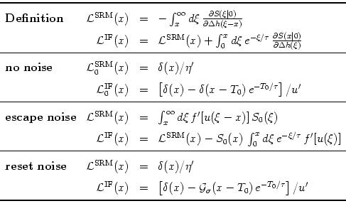
Table 7.1:
The kernel
(x) for integrate-and-fire
and SRM0 neurons (upper index IF and SRM, respectively) in the general
case (`Definition'), without noise, as well as for
escape and reset noise. S0(s) is the survivor function
in the asynchronous state and

 a normalized Gaussian with
width
a normalized Gaussian with
width  . Primes denote derivatives with respect to the
argument.
. Primes denote derivatives with respect to the
argument.
|
7.1.1 Noise-free Population Dynamics (*)
We start with a reduction of the population integral equation (6.75)
to the noise-free case. In the limit of no noise, the input-dependent
interval distribution
PI(t | ) reduces to a Dirac
function, i.e.,
PI(t | ) =  [t - - T()] . [t - - T()] . |
(7.5) |
where
T() is the inter-spike interval of a neuron that has fired its
last spike at time .
If we insert Eq. (7.5) in the integral equation of the population
activity,
A(t) = PI(t|) A() d,
we find
| A(t) = (t - - T()) A() d . |
(7.6) |
The interval
T() of a noise-free neuron is given implicitly by the
threshold condition
T() = min{(t - ) | u(t) =  ; ; > 0, t > } . > 0, t > } . |
(7.7) |
Note that
T() is the interval starting at and looking
forward towards the next spike; cf. Fig. 7.1. The
integration over the -function in Eq. (7.6) can be done, but
since T in the argument of the -function depends upon , the
evaluation of the integral needs some care.
Figure 7.1:
A neuron that has fired at time fires its next spike at
+ T() where T is the `forward' interval. Looking backwards we
find that a neuron that fires now at time t has fired its last spike at
t - Tb(t) where Tb is the backward interval.
![\hbox{\hspace{20mm}
\includegraphics[width=60mm]{Figs-ch-signal/forward-back.eps}}](img1158.gif) |
We recall from the rules for functions that
if f has a single zero-crossing
f (x0) = 0 in the interval a < x0 < b with
f'(x0) 0. The prime denotes the derivative. If there is no solution
f (x0) = 0 in the interval [a, b], the integral vanishes. In our case,
x plays the role of the variable with
f () = t - - T().
Hence
f'() = - 1 - T'() and
0. The prime denotes the derivative. If there is no solution
f (x0) = 0 in the interval [a, b], the integral vanishes. In our case,
x plays the role of the variable with
f () = t - - T().
Hence
f'() = - 1 - T'() and
A(t) =  A() , A() , |
(7.9) |
whenever a solution of
= t - Tb(t) exists. Here Tb(t) is the backward interval of neurons that reach the threshold at time t.
Eq. (7.9) allows an intuitive interpretation. The activity at
time t is proportional to the number of neurons that have fired one period
earlier. The proportionality constant is called compression factor. If
the inter-spike intervals decrease (T' < 0), then neuronal firing times are
`compressed' and the population activity increases. If inter-spike intervals
become larger (T' > 0), the population activity decreases;
cf. Fig. 7.2.
To evaluate
T'() we use the threshold condition (7.7).
From
 = u[ + T()] =
  [T()] + h[ + T()|] we find by taking the derivative with respect
to
[T()] + h[ + T()|] we find by taking the derivative with respect
to
0 =  [T()] T'() + [T()] T'() +  h[ + T()|] [1 + T'()] + h[ + T()|] [1 + T'()] +  h[ + T()|] . h[ + T()|] . |
(7.10) |
The prime denotes the derivative with respect to the argument. We have
introduced a short-hand notation for the
partial derivatives, viz.,
 h(t|) =
  h(t|)/t and
 h(t|) = h(t|)/.
We solve for T' and find
h(t|) = h(t|)/.
We solve for T' and find
T' = -  , , |
(7.11) |
where we have suppressed the arguments for brevity. A simple algebraic
transformation yields
 = 1 + = 1 +  , , |
(7.12) |
which we insert into Eq. (7.9). The result is
A(t) =  1 + 1 + 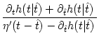 ![$\displaystyle \left.\vphantom{1 + {\partial_t h(t\vert\hat{t}) + \partial_{\hat...
...hat{t}) \over \eta'(t-\hat{t}) - \partial_{\hat{t}}h(t\vert\hat{t}) \,}}\right]$](img1172.gif) A() , with = t - Tb(t) , A() , with = t - Tb(t) , |
(7.13) |
where Tb(t) is the backward interval given a spike at time t. A
solution Tb(t) exists only if some neurons reach the threshold at time t.
If this is not the case, the activity A(t) vanishes. The partial
derivatives in Eq. (7.13) are to be evaluated at
= t - Tb(t);
the derivative
 = d(s)/ds is to be evaluated at
s = Tb(t).
We may summarize Eq. (7.13) by saying that the activity at time t
depends on the activity one period earlier modulated by the factor
in square brackets. Note that Eq. (7.13) is still
exact.
= d(s)/ds is to be evaluated at
s = Tb(t).
We may summarize Eq. (7.13) by saying that the activity at time t
depends on the activity one period earlier modulated by the factor
in square brackets. Note that Eq. (7.13) is still
exact.
Let us consider a fluctuating input current that generates small perturbations
in the population activity
A(t) and the input potential
h(t)
as outlined at the beginning of this section. If we substitute
A(t) = A0 + A(T) and
h(t|) = h0 + h(t|) into
Eq. (7.13) and linearize in A and h we obtain an
expression of the form
| A(t) = A(t - T) + A0 C(t) , |
(7.14) |
where T = 1/A0 is the interval for constant input I0 and C a
time-dependent factor, called compression factor. The activity
at time t depends thus on the activity one inter-spike interval earlier and
on the instantanuous value of the compression factor.
For SRM0 neurons we have
h(t|) = h(t) so that the partial
derivative with respect to vanishes. The factor in square brackets in
Eq. (7.13) reduces therefore to
[1 + (h'/)]. If we linearize
Eq. (7.13) we find
the compression factor
| CSRM(t) = h'(t)/(T) . |
(7.15) |
For integrate-and-fire neurons we have a similar result. To evaluate the
partial derivatives that we need in Eq. (7.13) we write
u(t) = (t - ) + h(t|) with
 (t - ) (t - ) |
= |
ur e |
|
| h(t|) |
= |
h(t) - h() e ; |
(7.16) |
cf. Eqs. (4.34) and (4.60).
Here ur is the reset potential of the integrate-and-fire neurons
and
h(t)
=  exp(- s/
 ) I(t - s) ds
is the input potential generated by the input current I.
) I(t - s) ds
is the input potential generated by the input current I.
Taking the derivative of and the partial derivatives of h yields
 = = ![$\displaystyle {h'(t) - h'(t-T_b) \, e^{-T_b/\tau_m} \over h' (t-T_b)\,e^{-T_b/\tau_m} - \tau_m^{-1}\,[u_r + h(t-T_b)] \, e^{-T_b/\tau_m}}$](img1176.gif) , , |
(7.17) |
which we now insert in Eq. (7.13). Since we are interested in the
linearized activity equation, we replace Tb(t) by the interval
T = 1/A0 for constant input and drop the term h' in the denominator. This
yields Eq. (7.14) with a compression factor
CIF given by
CIF(t) = [h'(t) - h'(t - T) exp(- T/ )]/u' . )]/u' . |
(7.18) |
Here
u' is the derivative of the membrane potential
for constant input current I0, i.e.,
u' = -  [ur + h(t - Tb)] e-Tb/
 .
The label IF is short for integrate-and-fire neurons.
.
The label IF is short for integrate-and-fire neurons.
In order to motivate the name `compression factor' and to give an
interpretation of Eq. (7.14) we consider SRM0
neurons with an exponential refractory kernel
(s) = -  exp(- s/
 ). We want to show graphically that the population
activity A has a contribution that is proportional to the derivative of the input potential.
). We want to show graphically that the population
activity A has a contribution that is proportional to the derivative of the input potential.
Figure 7.2:
A change in the input potential h
with positive slope h' > 0 (dashed line, bottom)
shifts neuronal firing times closer together
(middle).
As a result, the activity A(t) (solid line, top) is higher
at
t = + T() than it was at time
(schematic diagram); taken from (Gerstner, 2000b)
![\hbox{\hspace{20mm}
\includegraphics[width=60mm]{Figs-ch-signal/fig03.eps}}](img1177.gif) |
We consider Fig. 7.2. A neuron which has fired at will
fire again at
t = + T(). Another neuron which has fired
slightly later at
+ fires its next spike at
t + t.
If the input potential is constant between t and
t + t, then
t = . If, however, h increases between t and
t + t
as is the case in Fig. 7.2, then the firing time difference is
reduced. The compression of firing time differences is directly related to an
increase in the activity A. To see this, we note that all neurons which
fire between and
+ , must fire again between
t and
t + t. This is due to the fact that the network is homogeneous
and the mapping
 t = + T() is monotonous. If firing
time differences are compressed, the population activity increases.
t = + T() is monotonous. If firing
time differences are compressed, the population activity increases.
In order to establish the relation between
Fig. 7.2 and
Eq. (7.15),
we note that the compression faction is
equal to h'/.
For a SRM0 neuron with exponential refractory kernel,
(s) > 0 holds for all s > 0.
An input with h' > 0 implies then, because of
Eq. (7.14),
an increase of the activity:
h' > 0  A(t) > A(t - T) . A(t) > A(t - T) . |
(7.19) |
7.1.2 Escape noise (*)
In this section we focus on a population of neurons
with escape noise.
The aim of this section is two-fold. First, we want to show how to derive the
linearized population equation (7.3) that has
already been stated at the beginning of Section 7.1.
Second, we will show that in the case of high noise the population activity
follows the input potential h(t), whereas for low noise the activity follows
the derivative h'(t). These results will be used in the following three
sections for a discussion of signal transmission and coding properties.
In order to derive the linearized response A of the population
activity to a change in the input we start from the conservation law,
| 1 = SI(t | ) A() d , |
(7.20) |
cf. (6.73). As we have seen in Chapter 6.3
the population equation (6.75) can be obtained by taking the
derivative of Eq. (7.20) with respect to t, i.e.,
| 0 = SI(t | ) A() d . |
(7.21) |
For constant input I0, the population activity has a constant value
A0. We consider a small perturbation of the stationary state,
A(t) = A0 + A(t), that is caused by a small change in the input current,
I(t). The time-dependent input generates a total postsynaptic potential,
| h(t|) = h0(t|) + h(t|) , |
(7.22) |
where
h0(t|) is the postsynaptic potential for constant
input I0 and
| h(t|) = (t - , s) I(t - s) ds |
(7.23) |
is the change of the postsynaptic potential generated by I. We
expand Eq. (7.21) to linear order in A and h and
find
We have used the notation
S0(t - ) = SI0(t | ) for the survivor function of the asynchronous firing state.
To take the derivative of the first term in Eq. (7.24) we use
dS0(s)/ds = - P0(s) and S0(0) = 1. This yields
We note that the first term on the right-hand side of
Eq. (7.25) has the same form as the population integral equation
(6.75), except that P0 is the interval distribution in the
stationary state of asynchronous firing.
To make some progress in the treatment of the second term on the right-hand
side of Eq. (7.25), we restrict the choice of neuron model and focus on
SRM0 or integrate-and-fire neurons. For SRM0 neurons, we may drop the
dependence of the potential and set
h(t|) = h(t) where h is the input potential caused by the
time-dependent current I; compare Eqs. (7.4) and
(7.23). This allows us to pull the variable
h(s) in
front of the integral over and write Eq. (7.25) in the form
A(t) = P0(t - ) A() d + A0  (x) h(t - x) dx (x) h(t - x) dx . . |
(7.24) |
with a kernel
(x) = -  d d   SRM(x) ; SRM(x) ; |
(7.25) |
cf. Tab. 7.1.
For integrate-and-fire neurons we set
h(t|) = h(t) - h() exp[- (t - )/];
cf. Eq. (7.16). After some rearrangements of
the terms, Eq. (7.25) becomes identical to Eq. (7.26) with a
kernel
(x) = - d +  d e- d e- / /  IF(x) ; IF(x) ; |
(7.26) |
cf. Tab. 7.1.
Let us discuss Eq. (7.26). The first term on the right-hand side of
Eq. (7.26) is of the same form as the dynamic equation (6.75) and
describes how perturbations
A() in the past influence the
present activity
A(t). The second term gives an additional
contribution which is proportional to the derivative of a filtered
version of the potential h.
We see from Fig. 7.3
that the width of the kernel
depends on the noise level.
For low noise, it is significantly sharper than for high noise.
For a further discussion of Eq. (7.26)
we approximate the kernel by an exponential
low-pass filter
SRM(x) = a  e- e- x x  (x) , (x) , |
(7.27) |
where a is a constant and  is a measure of the noise.
It is shown in the examples below that
Eq. (7.29) is exact for neurons
with step-function escape noise and for neurons
with absolute refractoriness.
is a measure of the noise.
It is shown in the examples below that
Eq. (7.29) is exact for neurons
with step-function escape noise and for neurons
with absolute refractoriness.
The noise-free
threshold process can be retrieved from Eq. (7.29) for
 .
In this limit
SRM(x) = a (x) and the initial transient
is proportional to h' as discussed above. For small , however, the
behavior is different. We use Eq. (7.29) and rewrite the last term in
Eq. (7.26) in the form
.
In this limit
SRM(x) = a (x) and the initial transient
is proportional to h' as discussed above. For small , however, the
behavior is different. We use Eq. (7.29) and rewrite the last term in
Eq. (7.26) in the form
SRM(x) h(t - x) dx = a [h(t) -  (t)] (t)] |
(7.28) |
where
 (t) = exp(- x) h(t - x) dx is a running average. Thus the activity responds to the
temporal contrast
h(t) - (t). At high noise
levels is small so that
is an average over a long
time window; cf. Eq. (7.29). If the fluctuations I have
vanishing mean (
(t) = exp(- x) h(t - x) dx is a running average. Thus the activity responds to the
temporal contrast
h(t) - (t). At high noise
levels is small so that
is an average over a long
time window; cf. Eq. (7.29). If the fluctuations I have
vanishing mean (
 I
I = 0), we may set
(t) = 0. Thus, we find for escape noise in the large noise limit
A(t)
= 0), we may set
(t) = 0. Thus, we find for escape noise in the large noise limit
A(t)  h(t). This is exactly the result that would be expected for a
simple rate model.
h(t). This is exactly the result that would be expected for a
simple rate model.
Figure 7.3:
Interval distribution (A) and the kernel
SRM(x) (B) for SRM0 neurons with escape noise. The escape rate has been taken
as piecewise linear
=  [u - ]
 (u - ). For
low noise (solid lines in A and B) the interval distribution is sharply
peaked and the kernel
SRM has a small width. For high
noise (dashed line) both the interval distribution and the kernel
SRM are broad. The value of the bias current I0 has
been adjusted so that the mean interval is always 40ms.
The kernel has been normalized to
(x) dx = 1.
(u - ). For
low noise (solid lines in A and B) the interval distribution is sharply
peaked and the kernel
SRM has a small width. For high
noise (dashed line) both the interval distribution and the kernel
SRM are broad. The value of the bias current I0 has
been adjusted so that the mean interval is always 40ms.
The kernel has been normalized to
(x) dx = 1.
![\vbox{
\vspace{5mm}
\hbox{
{\bf A}
\hspace{70mm}
{\bf B}
}
\par\hbox{
\hs...
...ncludegraphics[height=30mm,width=45mm]{Figs-ch-signal/FilterL40-norm.eps}
}
}](img1189.gif) |
In the escape noise model, the survivor function is given by
SI(t | ) = exp![$\displaystyle \left\{\vphantom{ -\int_{\hat{t}}^t f[\eta(t'-\hat{t}) + h(t'\vert\hat{t}) ]\, {\text{d}} t' }\right.$](img1190.gif) - -  f[(t' - ) + h(t'|)] dt' f[(t' - ) + h(t'|)] dt'![$\displaystyle \left.\vphantom{ -\int_{\hat{t}}^t f[\eta(t'-\hat{t}) + h(t'\vert\hat{t}) ]\, {\text{d}} t' }\right\}$](img1191.gif) |
(7.29) |
where f[u] is the instantaneous escape rate across the noisy threshold;
cf. Chapter 5. We write
h(t|) = h0(t - ) + h(t|). Taking the derivative with respect to h yields
   = - (s - ) (t - s) f'[(s - ) + h0(s - )] S0(t - ) = - (s - ) (t - s) f'[(s - ) + h0(s - )] S0(t - ) |
(7.30) |
where
S0(t - ) = Sh0(t | ) and
f' = df (u)/du. For
SRM0-neurons, we have
h0(t - )  h0 and
h(t|) = h(t), independent of . The kernel
is therefore
h0 and
h(t|) = h(t), independent of . The kernel
is therefore
SRM(t - s) = (t - s) d f'[(s - ) + h0] S0(t - ) . d f'[(s - ) + h0] S0(t - ) . |
(7.31) |
as noted in Tab. 7.1.
Figure 7.4:
Interval distribution (A) and the kernel
IF(x) (B) for integrate-and-fire neurons with escape noise. The escape rate has
been taken as piecewise linear
= [u - ](u - ). The value of the bias current
I0 has been adjusted so that the mean interval is always 8ms. The
dip in the kernel around x = 8ms is typical for integrate-and-fire
neurons. Low noise: sharply peaked interval distribution and kernel.
High noise: broad interval distribution and kernel.
![\vbox{
\vspace{5mm}
\hbox{
{\bf A}
\hspace{70mm}
{\bf B}
}
\par\hbox{
\hs...
...cludegraphics[height=30mm,width=45mm]{Figs-ch-signal/FilterL8-IF.eps}
}
\par }](img1196.gif) |
We take
f (u) = (u - ), i.e.,
a step-function escape rate. For
neurons fire
immediately as soon as
u(t) > and we are back to the noise-free
sharp threshold. For finite , neurons respond stochastically with time
constant  .
We will show that the kernel
(x) for neurons
with step-function escape rate is an exponential function;
cf. Eq. (7.29).
.
We will show that the kernel
(x) for neurons
with step-function escape rate is an exponential function;
cf. Eq. (7.29).
Let us denote by T0 the time between the last firing time and the
formal threshold crossing,
T0 = min s | (s) + h0 =
  . The derivative of f is a
-function,
. The derivative of f is a
-function,
f'[(s) + h0] = [(s) + h0 - ] =  (s - T0) (s - T0) |
(7.32) |
where
=  |s=T0. The survivor function
S0(s) is
unity for s < T0 and
S0(s) = exp[- (s - T0)] for s > T0.
Integration of Eq. (7.33) yields
|s=T0. The survivor function
S0(s) is
unity for s < T0 and
S0(s) = exp[- (s - T0)] for s > T0.
Integration of Eq. (7.33) yields
(s) =  (s) exp[- (s)] (s) exp[- (s)] |
(7.33) |
as claimed above.
We take an arbitrary escape rate f (u) 0 with
limu
0 with
limu -
- f (u) = 0 = limu-f'(u). Absolute refractoriness is defined
by a refractory kernel
(s) = - for
0 < s <
f (u) = 0 = limu-f'(u). Absolute refractoriness is defined
by a refractory kernel
(s) = - for
0 < s <  and zero
otherwise. This yields
f[(t - ) + h0] = f (h0) (t - - ) and hence
and zero
otherwise. This yields
f[(t - ) + h0] = f (h0) (t - - ) and hence
f'[(t - ) + h0] = f'(h0) (t - -  ) . ) . |
(7.34) |
The survivor function S0(s) is unity for
s <
and decays as
exp[- f (h0) (s - )] for
s > .
Integration of Eq. (7.33) yields
(t - t1) = (t - t1) exp[- f (h0) (t - t1)] . exp[- f (h0) (t - t1)] . |
(7.35) |
Note that for neurons with absolute refractoriness the transition to the
noiseless case is not meaningful. We have seen in
Chapter 6 that absolute refractoriness leads to the
Wilson-Cowan integral equation (6.76). Thus
defined in
(7.37) is the kernel relating to Eq. (6.76); it could have
been derived directly from the linearization of the Wilson-Cowan integral
equation. We note that it is a low-pass filter with cut-off frequency
f (h0) which depends on the input potential h0.
We consider SRM0-neurons with noisy reset as introduced in
Chapter 5.4. After each spike the membrane potential is
reset to a randomly chosen value
parameterized by the reset variable r. This is an example of a `slow' noise model,
since a new value of the stochastic variable r is chosen
only once per inter-spike interval. The
interval distribution of the noisy reset model is
PI(t|) =  dr [t - - T(, r)] dr [t - - T(, r)]  (r) , (r) , |
(7.36) |
where
is a normalized Gaussian with width ; cf. Eq. (5.68). The population equation
(6.75) is thus
| A(t) = ddr [t - - T(, r)] (r) A() . |
(7.37) |
A neuron that has been reset at time with value r
behaves identical to a noise-free neuron that has fired its last spike
at
+ r.
In particular we have the relation
T(, r) = r + T0( + r) where T0(t') is the forward
interval of a noiseless neuron that has fired its last spike at t'.
The
integration over in Eq. (7.39) can
therefore be done and yields
A(t) =  1 + 1 +  ![$\displaystyle \left.\vphantom{1+{h'\over \eta'}}\right]$](img1208.gif) dr (r) A[t - Tb(t) - r] dr (r) A[t - Tb(t) - r] |
(7.38) |
where Tb is the backward interval. The factor
[1 + (h'/)] arises due
to the integration over the -function just as in the noiseless case;
cf. Eqs. (7.13) and (7.15).
To simplify the expression, we write
A(t) = A0 + A(t) and expand
Eq. (7.40) to first order in A. The result is
A(t) = (r) A(t - T0 - r) dr +  A0 A0 |
(7.39) |
A comparison of Eqs. (7.41) and (7.3) yields the kernel
(x) = (x)/ for the noisy-reset model. Note that it is
identical to that of a population of noise-free neurons;
cf. Tab. 7.1.
The reason is that the effect of noise is limited to the moment
of the reset. The approach of the membrane potential
towards the threshold is noise-free.
Next: 7.2 Transients
Up: 7. Signal Transmission and
Previous: 7. Signal Transmission and
Gerstner and Kistler
Spiking Neuron Models. Single Neurons, Populations, Plasticity
Cambridge University Press, 2002
© Cambridge University Press
This book is in copyright. No reproduction of any part
of it may take place without the written permission
of Cambridge University Press.