In this section, we derive, starting from a small set of assumptions, an
integral equation for the population activity. The essential idea of the
mathematical formulation is that we work as much as possible on the
macroscopic level without reference to a specific model of neuronal dynamics.
We will see that the interval distribution
PI(t|![]() ) that has already
been introduced in Chapter 5 plays a central role in the
formulation of the population equation. Both the activity variable A and
the interval distribution
PI(t|
) that has already
been introduced in Chapter 5 plays a central role in the
formulation of the population equation. Both the activity variable A and
the interval distribution
PI(t|![]() ) are `macroscopic' spike-based
quantities that could, in principle, be measured by extracellular electrodes.
If we have access to the interval distribution
PI(t|
) are `macroscopic' spike-based
quantities that could, in principle, be measured by extracellular electrodes.
If we have access to the interval distribution
PI(t|![]() ) for arbitrary
input I(t), then this knowledge is enough to formulate the population
equations. In particular, there is no need to know anything about the
internal state of the neuron, e.g., the current values of the membrane
potential of the neurons.
) for arbitrary
input I(t), then this knowledge is enough to formulate the population
equations. In particular, there is no need to know anything about the
internal state of the neuron, e.g., the current values of the membrane
potential of the neurons.
Integral formulations of the population dynamics have been developed by (Gerstner, 1995,2000b; Wilson and Cowan, 1972; Gerstner and van Hemmen, 1992; Knight, 1972a). The integral equation (6.44) that we have derived in Section 6.2 via integration of the density equations turns out to be a specific instance of the general framework presented in this section.
We consider a homogeneous and fully connected
network of spiking neurons in the limit
of
N![]()
![]() .
We aim for a dynamic equation that
describes the evolution of the population activity A(t)
over time.
.
We aim for a dynamic equation that
describes the evolution of the population activity A(t)
over time.
We have seen in Eq. (6.8) that,
given the population activity A(t')
and the external input
Iext(t') in the past,
we can calculate the current input potential
hPSP(t|![]() )
of a neuron that has fired its last spike at
)
of a neuron that has fired its last spike at ![]() ,
but we have no means yet to transform the
potential
hPSP back into a population activity.
What we need is therefore another equation which allows us to
determine the present activity A(t) given
the past.
The equation for the activity dynamics
will be derived from three observations:
,
but we have no means yet to transform the
potential
hPSP back into a population activity.
What we need is therefore another equation which allows us to
determine the present activity A(t) given
the past.
The equation for the activity dynamics
will be derived from three observations:
Because of observation (ii) we know that the input-dependent interval
distribution
PI(t | ![]() ) contains all relevant information.
We recall that
PI(t |
) contains all relevant information.
We recall that
PI(t | ![]() ) gives
the probability density that a neuron fires at time t
given its last spike at
) gives
the probability density that a neuron fires at time t
given its last spike at ![]() and an input I(t') for t' < t.
Integration of the probability density
over time
and an input I(t') for t' < t.
Integration of the probability density
over time
![]() PI(s |
PI(s | ![]() ) ds
gives the probability
that a neuron which has fired at
) ds
gives the probability
that a neuron which has fired at ![]() fires its next spike at some arbitrary time between
fires its next spike at some arbitrary time between
![]() and t. Just as in Chapter 5,
we can define
a survival probability,
and t. Just as in Chapter 5,
we can define
a survival probability,
We now return to the homogeneous population of neurons
in the limit of
N![]()
![]() and use
observation (iii).
We consider the network state at time t
and label all neurons by their last firing time
and use
observation (iii).
We consider the network state at time t
and label all neurons by their last firing time ![]() .
The proportion of neurons at time t which have fired
their last spike between
t0 and t1 < t (and have not fired since) is expected to be
.
The proportion of neurons at time t which have fired
their last spike between
t0 and t1 < t (and have not fired since) is expected to be
For an interpretation of the integral
on the right-hand side of Eq. (6.72), we recall
that
A(![]() )
)![]()
![]() is the fraction
of neurons that have fired in the interval
[
is the fraction
of neurons that have fired in the interval
[![]() ,
,![]() +
+ ![]()
![]() ].
Of these a fraction
SI(t|
].
Of these a fraction
SI(t|![]() ) are expected
to survive from
) are expected
to survive from ![]() to t without firing.
Thus among the neurons that we observe at time t
the proportion of neurons that have fired their
last spike between t0 and t1 is
expected to be
to t without firing.
Thus among the neurons that we observe at time t
the proportion of neurons that have fired their
last spike between t0 and t1 is
expected to be
![]() SI(t |
SI(t | ![]() ) A(
) A(![]() ) d
) d![]() ;
cf. Fig. 6.7.
;
cf. Fig. 6.7.
![\hbox{\hspace{20mm}
\includegraphics[width=80mm]{Figs-ch-pop/pop-surv.eps}}](img1082.gif) |
Finally, we make use of observation (i).
All neurons have fired at some point in
the past6.2. Thus, if we extend the lower bound
t0 of the integral on the right-hand side
of Eq. (6.72) to - ![]() and the upper bound to t,
the left-hand side becomes equal to one,
and the upper bound to t,
the left-hand side becomes equal to one,
Since Eq. (6.73) is rather abstract, we try to put it into a form that is easier to grasp intuitively. To do so, we take the derivative of Eq. (6.73) with respect to t. We find
0 = SI(t| t) A(t) +  A( A( |
(6.74) |
Eq. (6.75) is easy to understand.
The kernel
PI(t | ![]() ) is the probability density
that the next spike of a neuron which is
under the influence of an input I
occurs at time t given that its last
spike was at
) is the probability density
that the next spike of a neuron which is
under the influence of an input I
occurs at time t given that its last
spike was at ![]() .
The number of neurons which have fired at
.
The number of neurons which have fired at ![]() is proportional
to
A(
is proportional
to
A(![]() ) and the integral runs over all times in the past.
The interval distribution
PI(t|
) and the integral runs over all times in the past.
The interval distribution
PI(t|![]() ) depends upon the total
input (both external input and synaptic input
from other neurons in the population)
and hence upon the postsynaptic potential (6.8).
Eqs. (6.8) and (6.75) together
with an appropriate noise model yield
a closed system of equations for the population dynamics.
Eq. (6.75) is exact in the limit of
N
) depends upon the total
input (both external input and synaptic input
from other neurons in the population)
and hence upon the postsynaptic potential (6.8).
Eqs. (6.8) and (6.75) together
with an appropriate noise model yield
a closed system of equations for the population dynamics.
Eq. (6.75) is exact in the limit of
N![]()
![]() .
Corrections for finite N,
have been discussed by Meyer and van Vreeswijk (2001) and
Spiridon and Gerstner (1999).
.
Corrections for finite N,
have been discussed by Meyer and van Vreeswijk (2001) and
Spiridon and Gerstner (1999).
An important remark concerns the proper normalization
of the activity.
Since Eq. (6.75) is defined as the derivative
of Eq. (6.73), the integration constant on the left-hand side
of (6.73) is lost.
This is most easily seen for constant activity
A(t) ![]() A0.
In this case the variable A0
can be eliminated on both sides
of Eq. (6.75)
so that Eq. (6.75) yields the trivial
statement that the interval distribution is normalized to unity.
Equation
(6.75)
is therefore invariant under a rescaling
of the activity
A0
A0.
In this case the variable A0
can be eliminated on both sides
of Eq. (6.75)
so that Eq. (6.75) yields the trivial
statement that the interval distribution is normalized to unity.
Equation
(6.75)
is therefore invariant under a rescaling
of the activity
A0 ![]() c A0.
with any constant c.
To get the correct normalization
of the activity A0
we have to go back to
Eq. (6.73).
c A0.
with any constant c.
To get the correct normalization
of the activity A0
we have to go back to
Eq. (6.73).
We conclude this section
with a final remark on the form of Eq. (6.75).
Even though
(6.75) looks linear, it is in fact
a highly non-linear equation
because the kernel
PI(t | ![]() )
depends non-linearly on
hPSP, and
hPSP
in turn depends on
the activity via Eq. (6.8).
)
depends non-linearly on
hPSP, and
hPSP
in turn depends on
the activity via Eq. (6.8).
Let us consider a population of Poisson neurons with
an absolute refractory period
![]() .
A neuron that is not refractory,
fires stochastically with a rate f[h(t)]
where h(t) is the total input potential,
viz., the sum of the postsynaptic potentials
caused by presynaptic spike arrival.
After firing, a neuron is inactive
during the time
.
A neuron that is not refractory,
fires stochastically with a rate f[h(t)]
where h(t) is the total input potential,
viz., the sum of the postsynaptic potentials
caused by presynaptic spike arrival.
After firing, a neuron is inactive
during the time
![]() .
The population activity of
a homogeneous group of Poisson neurons
with absolute refractoriness is
(Wilson and Cowan, 1972)
.
The population activity of
a homogeneous group of Poisson neurons
with absolute refractoriness is
(Wilson and Cowan, 1972)
The Wilson-Cowan integral equation
(6.76) has a simple interpretation.
Neurons stimulated by a total postsynaptic potential
h(t) fire with an instantaneous rate f[h(t)].
If there were no refractoriness, we would
expect a population activity
A(t) = f[h(t)].
Not all neurons may, however, fire since some of the neurons are
in the absolute refractory period.
The fraction of neurons that participate in firing
is
1 - ![]() A(t') dt'
which explains the factor in curly brackets.
A(t') dt'
which explains the factor in curly brackets.
For constant input potential, h(t) = h0, the population activity has a stationary solution,
![\hbox{{\bf A} \hspace{65mm} {\bf B}}
\hbox{\hspace{10mm}
\includegraphics[width=...
...nf.eps}
\hspace{10mm}
\includegraphics[width=53mm]{Figs-ch-pop/WC-Abaroft.eps}}](img1092.gif) |
The function f in Eq. (6.76)
was motivated by an instantaneous `escape rate'
due to a noisy threshold
in a homogeneous population.
In this interpretation,
Eq. (6.76) is the exact equation for
the population activity of
neurons with absolute refractoriness.
In their original paper,
Wilson and Cowan motivated the function f
by a distribution of threshold values ![]() in an inhomogeneous population.
In this case, the population equation
(6.76) is an approximation,
since correlations are neglected
(Wilson and Cowan, 1972).
in an inhomogeneous population.
In this case, the population equation
(6.76) is an approximation,
since correlations are neglected
(Wilson and Cowan, 1972).
We apply the population equation
(6.75) to SRM0 neurons with
escape noise; cf. Chapter 5.
The escape rate
f (u - ![]() ) is
a function of the distance between the membrane
potential and the threshold. For the sake
of notational convenience, we set
) is
a function of the distance between the membrane
potential and the threshold. For the sake
of notational convenience, we set
![]() = 0.
The neuron model is specified by a refractory function
= 0.
The neuron model is specified by a refractory function ![]() as follows.
During an absolute refractory period
0 < s
as follows.
During an absolute refractory period
0 < s![]()
![]() ,
we set
,
we set ![]() (s) to -
(s) to - ![]() .
For
s
.
For
s![]()
![]() , we set
, we set
![]() (s) = 0.
Thus the neuron exhibits absolute refractoriness only;
cf. Eq. (5.57).
The total membrane potential is
u(t) =
(s) = 0.
Thus the neuron exhibits absolute refractoriness only;
cf. Eq. (5.57).
The total membrane potential is
u(t) = ![]() (t -
(t - ![]() ) + h(t)
with
) + h(t)
with
Given ![]() it seems natural to split the integral in the
activity equation (6.75) into two parts
it seems natural to split the integral in the
activity equation (6.75) into two parts
| PI(t | |
(6.80) |
Let us evaluate the two terms on the right-hand side of
Eq. (6.79).
Since
spiking is impossible during the absolute refractory time,
i.e.,
f[- ![]() ] = 0, the second term in Eq. (6.79)
vanishes.
In the first term we can move a factor
f[h(t) +
] = 0, the second term in Eq. (6.79)
vanishes.
In the first term we can move a factor
f[h(t) + ![]() (t -
(t - ![]() )] = f[h(t)]
in front of
the integral since
)] = f[h(t)]
in front of
the integral since ![]() vanishes for
t -
vanishes for
t - ![]() >
> ![]() .
The exponential factor is
the survivor function
of neurons with escape noise as
defined in Eq. (5.7); cf. Chapter 5.
Therefore Eq. (6.79) reduces to
.
The exponential factor is
the survivor function
of neurons with escape noise as
defined in Eq. (5.7); cf. Chapter 5.
Therefore Eq. (6.79) reduces to
Integral equations are often difficult to handle.
Wilson and Cowan aimed therefore at a transformation of
their equation into a differential equation
(Wilson and Cowan, 1972).
To do so, they had to assume that the
population activity changes slowly during the time
![]() and adopted a procedure of time coarse-graining.
Here we present a slightly modified version
of their argument (Pinto et al., 1996; Gerstner, 1995).
and adopted a procedure of time coarse-graining.
Here we present a slightly modified version
of their argument (Pinto et al., 1996; Gerstner, 1995).
We start with the observation that the total postsynaptic potential,
As a second step, we transform Eq. (6.85) into
a differential equation. If the response kernels are exponentials,
i.e.,
![]() (s) =
(s) = ![]() (s) =
(s) = ![]() exp(- s/
exp(- s/![]() ),
the derivative of Eq. (6.85) is
),
the derivative of Eq. (6.85) is
Equation (6.87) is a differential equation for the membrane potential. Alternatively, the integral equation (6.76) can also be approximated by a differential equation for the activity A. We start from the observation that in a stationary state the activity A can be written as a function of the input current, i.e, A0 = g(I0) where I0 = Iext + J0 A0 is the sum of the external driving current and the postsynaptic current caused by lateral connections within the population. What happens if the input current changes? The population activity of neurons with a large amount of escape noise will not react to rapid changes in the input instantaneously, but follow slowly with a certain delay similar to the characteristics of a low-pass filter. An equation that qualitatively reproduces the low-pass behavior is
The Wilson-Cowan integral equation that has been discussed above is valid for
neurons with absolute refractoriness only. We now generalize some of the
arguments to a Spike Response Model with relative refractoriness. We suppose
that refractoriness is over after a time
![]() so that
so that
![]() (s) = 0 for
s
(s) = 0 for
s![]()
![]() . For
0 < s <
. For
0 < s < ![]() , the
refractory kernel may have any arbitrary shape. Furthermore we assume that
for
t >
, the
refractory kernel may have any arbitrary shape. Furthermore we assume that
for
t > ![]() the kernels
the kernels
![]() (t -
(t - ![]() , s) and
, s) and
![]() (t -
(t - ![]() , s) do not depend on t -
, s) do not depend on t - ![]() . For
0 < t -
. For
0 < t - ![]() <
< ![]() we allow for an arbitrary time-dependence. Thus, the
postsynaptic potential is
we allow for an arbitrary time-dependence. Thus, the
postsynaptic potential is
We start from the population equation (6.75) and split the integral into two parts
The integrals on the right-hand side of (6.91) have finite support which makes Eq. (6.91) more convenient for numerical implementation than the standard formulation (6.75). For a rapid implementation scheme, it is convenient to introduce discretized refractory densities as discussed in Section 6.2; cf. Eq. (6.57).
© Cambridge University Press
This book is in copyright. No reproduction of any part
of it may take place without the written permission
of Cambridge University Press.
![$\displaystyle {{\text{number of neurons at $t$with last spike in}~[t_0,t_1]} \over {\text{total number of neurons}}}$](img1078.gif)
 A(t') dt'
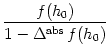 = g(h0) .
 PI(t |
 ![$\displaystyle {f[h(t)] \over 1 + \Delta^{\rm abs}\, f[h(t)]}$](img1099.gif) = : g[h(t)]
= : g[h(t)]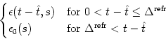 ,
, PI(t |
 PI(t |