Subsections

• 7.2.1 Transients in a Noise-Free Network
  • 7.2.1.1 Example: Initial transient of integrate-and-fire neurons
  
  
• 7.2.2 Transients with Noise
  • 7.2.2.1 Example: Response of neurons with escape noise
  • 7.2.2.2 Example: Slow response of standard rate model
  • 7.2.2.3 Example: Rapid response of neurons with `slow' noise
  • 7.2.2.4 Example: Diffusive noise

7.2 Transients

How quickly can a population of neurons respond to a rapid change in the input? We know from reaction time experiments that the response of humans and animals to new stimuli can be very fast (Thorpe et al., 1996). We therefore expect that the elementary processing units, i.e., neurons or neuronal populations should also show a rapid response. In this section we concentrate on one element of the problem of rapid reaction time and study the response of the population activity to a rapid change in the input. 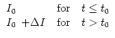To keep the arguments as simple as possible, we consider an input which has a constant value I₀ for t < t₀ and changes then abruptly to a new value I₀ + $\Delta$I. Thus

$$\left\{\vphantom{ \begin{array}{*{3}{c@{\quad}}c} I_0 && {\rm for... ...0 \\ I_0 &\!\!\!+ \Delta I& {\rm for } & t> t_0 \nonumber \end{array} }\right. \begin{array}{*{3}{c@{\quad}}c} I_0 && {\rm for} & t\le t_0 \\ I_0 &\!\!\!+ \Delta I& {\rm for } & t> t_0 \nonumber \end{array}$$

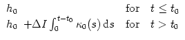
For the sake of simplicity, we consider a population of independent integrate-and-fire or SRM₀ neurons without lateral coupling. Given the current I^ext(t), the input potential can be determined from h(t) = $\int_{0}^{\infty}$$\kappa_{0}^{}$(s) I^ext(t - s) ds. For t$\le$t₀, the input potential has then a value h₀ = R I₀ where we have used $\int$$\kappa_{0}^{}$(s)ds = R. For t > t₀, the input potential h changes due to the additional current $\Delta$I so that

$$\left\{\vphantom{\begin{array}{*{3}{c@{\quad}}c} h_0 && {\rm for}... ...appa _0 (s) \, {\text{d}}s & {\rm for } & t> t_0 \nonumber \end{array} }\right. \begin{array}{*{3}{c@{\quad}}c} h_0 && {\rm for} & t\le t_0 \\ h... ...t-t_0} \kappa _0 (s) \, {\text{d}}s & {\rm for } & t> t_0 \nonumber \end{array}$$

Given the input potential h(t) and the last firing time $\hat{{t}}$ we can calculate for any given neuron its momentary membrane potential u(t) - but what is the time course of the population activity?

Let us suppose that for t < t₀ the network is in a state of asynchronous firing so that the population activity is constant, A(t) = A₀ for t$\le$t₀; cf. Chapter 6.4. As soon as the input is switched on at time t = t₀, the population activity will change

$$\Delta$$ (7.40)

In this section we will use the linear population equation,

$$\Delta \int_{{-\infty}}^{t} \hat{{t}} \Delta \hat{{t}} \hat{{t}} {{\text{d}}\over {\text{d}}t} \int_{0}^{\infty} \mathcal {L} \Delta$$ (7.41)

in order to calculate the linear response $\Delta$A(t) to the change in the input; cf. Eq. (7.3). Here P₀(t - $\hat{{t}}$) is the inter-spike interval distribution in the stationary state and $\mathcal {L}$(x) is the real-valued kernel given in Tab. 7.1. We are mainly interested in the initial phase of the transient, i.e. 0 < t - t₀ $\ll$ T where T = 1/A₀ is the mean inter-spike interval. During the initial phase of the transient, the first term on the right-hand side of Eq. (7.45) does not contribute, since $\Delta$A($\hat{{t}}$) = 0 for $\hat{{t}}$ < t₀. Therefore, Eq. (7.45) reduces to

$$\Delta {{\text{d}}\over {\text{d}}t} \int_{0}^{\infty} \mathcal {L} \Delta \ll$$ (7.42)

7.2.1 Transients in a Noise-Free Network

Figure 7.5: Top: Response of the population activity to a step current for very low noise. Solid line: simulation of a population of 1000 neurons. Dashed line: numerical integration of the population equation (6.75). A. integrate-and-fire-neurons; B. SRM₀ neurons. Bottom: step current input $\mathcal {I}$ (solid line) and input potential h(t) (dashed line). Note that the population responds instantaneously to the input switch at t₀ = 100 ms even though the membrane potential responds only slowly; taken from Gerstner (2000b)

In the noiseless case, neurons which receive a constant input I₀ fire regularly with some period T₀. For t < t₀, the mean activity is simply A₀ = 1/T₀. The reason is that, for a constant activity, averaging over time and averaging over the population are equivalent; cf. Chapter 6.4.

Let us consider a neuron which has fired exactly at t₀. Its next spike occurs at t₀ + T where T is given by the threshold condition u_i(t₀ + T) = $\vartheta$. We focus on the initial phase of the transient and apply the noise-free kernel $\mathcal {L}$(x) $\propto$ $\delta$(x); cf. Tab. 7.1. If we insert the $\delta$ function into Eq. (7.46) we find

$$\Delta \propto {{\text{d}}\over {\text{d}}t}$$ (7.43)

For both SRM₀ and integrate-and-fire neurons, the transient response is proportional to the derivative of the input potential h. Taking the derivative of Eq. (7.43) yields

$$\Delta \kappa_{0}^{}$$ (7.44)

with a constant a = R $\Delta$I/$\eta{^\prime}$ for SRM₀ neurons and a = R $\Delta$I/u' for integrate-and-fire neurons. Thus, the time course of the initial transient reflects the time course of the response kernel $\kappa_{0}^{}$. The initial transient of the neuronal response can therefore be extremely fast (Maršálek et al., 1997).

7.2.1.1 Example: Initial transient of integrate-and-fire neurons

In this example we apply Eq. (7.48) to integrate-and-fire neurons. The response kernel is

$$\kappa_{0}^{} {1\over \tau_m} \left(\vphantom{ -{s\over \tau_m}}\right. {s\over \tau_m} \left.\vphantom{ -{s\over \tau_m}}\right) \mathcal {H}$$ (7.45)

The response of the input potential to the step current (7.42) is

$$\Delta \left[\vphantom{1 - \exp\left(-{t-t_0\over \tau_m}\right)}\right. \left(\vphantom{-{t-t_0\over \tau_m}}\right. {t-t_0\over \tau_m} \left.\vphantom{-{t-t_0\over \tau_m}}\right) \left.\vphantom{1 - \exp\left(-{t-t_0\over \tau_m}\right)}\right]$$ (7.46)

which has the characteristics of a low-pass filter with time constant $\tau_{m}^{}$. The population activity, however, reacts instantaneously to the step current. We put the exponential kernel (7.49) in Eq. (7.48) and find

$$\Delta {a\, A_0 \over \tau_m} \left(\vphantom{-{t-t_0\over \tau_m}}\right. {t-t_0\over \tau_m} \left.\vphantom{-{t-t_0\over \tau_m}}\right) \mathcal {H}$$ (7.47)

where $\mathcal {H}$( ^. ) is the Heaviside step function. Thus, there is an immediate response at t = t₀. The simulation in Fig. 7.5 clearly exhibits the rapid initial response of the population. It is also confirmed by a numerical integration of the noise-free population equation; cf. Eq. (7.13).

A similar result holds for a population of SRM₀ neurons. The initial transient of SRM₀ is identical to that of integrate-and-fire neurons; cf. Fig. 7.5. A subtle difference, however, occurs during the late phase of the transient. For integrate-and-fire neurons the transient is over as soon as each neuron has fired once. After the next reset, all neurons fire periodically with a new period T that corresponds to the constant input I₀ + $\Delta$I. A population of SRM₀ neurons, however, reaches a periodic state only asymptotically. The reason is that the interspike interval T of SRM₀ neurons [which is given by the threshold condition h(t) = $\vartheta$ - $\eta_{0}^{}$(T)] depends on the momentary value of the input potential h(t).

7.2.2 Transients with Noise

Figure 7.6: A. Reset noise. Transients for SRM₀ neurons with noisy reset in response to the same step current as in Fig. 7.5. The results of a simulation of 1000 SRM₀-neurons (solid line) are compared with a numerical integration (dashed line) of the population integral equation; cf. Eq. (6.75). The instantaneous response is typical for `slow' noise models. B. Transients in a standard rate model. The new stationary state is approached exponentially with the membrane time constant $\tau_{m}^{}$. The response to the input switch at t₀ = 100ms is therefore comparatively slow.

So far, we have considered noiseless neurons. We have seen that after an initial sharp transient the population activity approaches a new periodic state where the activity oscillates with period T. In the presence of noise, we expect that the network approaches - after a transient - a new asynchronous state with stationary activity A₀ = g(I₀ + $\Delta$I); cf. Chapter 6.4.

In Fig. 7.6A illustrates the response of a population of noisy neurons to a step current input. The population activity responds instantaneously as soon as the additional input is switched on. Can we understand the sharply peaked transient? Before the abrupt change the input was stationary and the population in a state of asynchronous firing. Asynchronous firing was defined as a state with constant activity so that at any point in time some of the neurons fire, others are in the refractory period, again others approach the threshold. There is always a group of neuron whose potential is just below threshold. An increase in the input causes those neurons to fire immediately - and this accounts for the strong population response during the initial phase of the transient.

As we will see in the example below, the above consideration is strictly valid only for neurons with slow noise in the parameters, e.g., noisy reset as introduced in Chapter 5.4. In models based on the Wilson-Cowan differential equation the transient does not exhibit such a sharp initial peak; cf. Fig. 7.6B.

For diffusive noise models the picture is more complicated. A rapid response occurs if the current step is sufficiently large and the noise level not too high. On the other hand, for high noise and small current steps the response is slow. The question of whether neuronal populations react rapidly or slowly depends therefore on many aspects, in particular on the type of noise and the type of stimulation. It can be shown that for diffusive noise that is low-pass filtered by a slow synaptic time constant (i.e., cut-off frequency of the noise lower than the neuronal firing rate) the response is sharp, independent of the noise amplitude. On the other hand, for white noise the response depends on the noise amplitude and the membrane time constant (Brunel et al., 2001).

For a mathematical discussion of the transient behavior, it is sufficient to consider the equation that describes the initial phase of the linear response to a sudden onset of the input potential; cf. Eq. (7.46). Table 7.1 summarizes the kernel $\mathcal {L}$(x) that is at the heart of Eq. (7.46) for several noise models. In the limit of low noise, the choice of noise model is irrelevant - the transient response is proportional to the derivative of the potential, $\Delta$A $\propto$ h'. If the level of noise is increased, a population of neurons with slow noise (e.g., with noisy reset) retains its sharp transients since the kernel $\mathcal {L}$ is proportional to h',

Neurons with escape noise turn in the high-noise limit to a different regime where the transients follow h rather than h'. To see why, we recall that the kernel $\mathcal {L}$ essentially describes a low-pass filter; cf. Fig. 7.3. The time constant of the filter increases with the noise level and hence the response switches from a behavior proportional to h' to a behavior proportional to h.

7.2.2.1 Example: Response of neurons with escape noise

The width of the kernel $\mathcal {L}$(x) in Eq. (7.46) depends on the noise level. For low noise, the kernel is sharply peaked at x = 0 and can be approximated by a Dirac $\delta$ function. The response $\Delta$A of the population activity is sharp since it is proportional to the derivative of the input potential.

For high noise, the kernel is broad and the response becomes proportional to the input potential; cf. Fig. 7.7.

Figure 7.7: Escape noise. Response of a network of 1000 SRM₀ neurons with exponential escape noise to step current input. The input is switched at t = 100 ms. Simulations (fluctuating solid line) are compared to the numerical integration of the population equation (thick dashed line). A. For low noise the transition is comparatively sharp. B. For high noise the response to the change in the input is rather smooth.

7.2.2.2 Example: Slow response of standard rate model

In Chapter 6.3, we have introduced the Wilson-Cowan differential equations which are summarized here for a population of independent neurons,

A(t) = g[h(t)] ,

$$\tau_{m}^{} {{\text{d}}h\over {\text{d}}t}$$ = - h(t) + R I^ext(t) ; (7.48)

cf. Eq. (6.87). A step current input, causes a potential

$$\Delta \left[\vphantom{1 - \exp\left(-{t-t_0\over \tau_m}\right)}\right. \left(\vphantom{-{t-t_0\over \tau_m}}\right. {t-t_0\over \tau_m} \left.\vphantom{-{t-t_0\over \tau_m}}\right) \left.\vphantom{1 - \exp\left(-{t-t_0\over \tau_m}\right)}\right] \mathcal {H}$$ (7.49)

The response of the population activity is therefore

$$\Delta \Delta \left[\vphantom{1 - \exp\left(-{t-t_0\over \tau_m}\right)}\right. \left(\vphantom{-{t-t_0\over \tau_m}}\right. {t-t_0\over \tau_m} \left.\vphantom{-{t-t_0\over \tau_m}}\right) \left.\vphantom{1 - \exp\left(-{t-t_0\over \tau_m}\right)}\right] \mathcal {H}$$ (7.50)

where g' = dg/dh evaluated at h₀. Equation (7.54) describes a slow exponential response with time constant $\tau_{m}^{}$; cf. Fig. 7.6B. The Wilson-Cowan differential equation is a reasonable approximation for neurons with a large level of escape noise; compare Figs. 7.6B and 7.7B.

7.2.2.3 Example: Rapid response of neurons with `slow' noise

For neurons with noisy reset, the kernel $\mathcal {L}$ is a Dirac $\delta$ function; cf. Tab. 7.1. As in the noiseless case, the initial transient is therefore proportional to the derivative of h. After this initial phase the reset noise leads to a smoothing of subsequent oscillations so that the population activity approaches rapidly a new asynchronous state; cf. Fig. 7.6A. The initial transient, however, is sharp.

7.2.2.4 Example: Diffusive noise

In this example, we present qualitative arguments to show that, in the limit of low noise, a population of spiking neurons with diffusive noise will exhibit an immediate response to a strong step current input. We have seen in the noise-free case, that the rapid response is due the derivative h' in the compression factor. In order to understand, why the derivative of h comes into play, let us consider, for the moment, a finite step in the input potential h(t) = h₀ + $\Delta$h $\mathcal {H}$(t - t₀). All neurons i which are hovering below threshold so that their potential u_i(t₀) is between $\vartheta$ - $\Delta$h and $\vartheta$ will be put above threshold and fire synchronously at t₀. Thus, a step in the potential causes a $\delta$-pulse in the activity $\Delta$A(t) $\propto$ $\delta$(t - t₀) $\propto$ h'(t₀). In Fig. 7.8a we have used a current step (7.42) [the same step current as in Fig. 7.5]. The response at low noise (top) has roughly the form $\Delta$A(t) $\propto$ h'(t) $\propto$ $\kappa_{0}^{}$(t - t₀) as expected. The rapid transient is slightly less pronounced than for noisy reset, but nevertheless clearly visible; compare Figs. 7.6A and 7.8A. As the amplitude of the noise grows, the transient becomes less sharp. Thus there is a transition from a regime where the transient is proportional to h' (Fig. 7.8A) to another regime where the transient is proportional to h (Fig. 7.8B). What are the reasons for the change of behavior?

The simple argument from above based on a potential step $\Delta$h > 0 only holds for a finite step size which is at least of the order of the noise amplitude $\sigma$. With diffusive noise, the threshold acts as an absorbing boundary. Therefore the density of neurons with potential u_i vanishes for u_i$\to$$\vartheta$; cf. Chapter 6.2. Thence, for $\Delta$h$\to$ 0 the proportion of neurons which are instantaneously put across threshold is 0. In a stationary state, the 'boundary layer' with low density is of the order $\sigma$; e.g., cf. Eq. (6.28). A potential step $\Delta$h > $\sigma$ puts a significant proportion of neurons above threshold and leads to a $\delta$-pulse in the activity. Thus the result that the response is proportional to the derivative of the potential is essentially valid in the low-noise regime.

Figure 7.8: Diffusive Noise. Response of a network of 1000 integrate-and-fire neurons with diffusive noise to step current input. Simulations (fluctuating solid line) are compared to a numerical integration of the density equations (thick dashed line). A. For low noise and a big (super-threshold) current step the response is rapid. B. For high noise and a small current step the response is slow.

On the other hand, we may also consider diffusive noise with large noise amplitude in the sub-threshold regime. In the limit of high noise, a step in the potential raises the instantaneous rate of the neurons, but does not force them to fire immediately. The response to a current step is therefore smooth and follows the potential h(t); cf.  Fig. 7.8B. A comparison of Figs. 7.8 and 7.7 shows that the escape noise model exhibits a similar transition form sharp to smooth responses with increasing noise level. In fact, we have seen in Chapter 5 that diffusive noise can be well approximated by escape noise (Plesser and Gerstner, 2000). For the analysis of response properties with diffusive noise see Brunel et al. (2001).